How do I correct a measurement with them?
Microphone specifications may contain a group of specs related to microphone behavior under different environmental conditions. These are the environmental specifications, and they are usually presented as environmental coefficients. These specifications are typically forgotten or misunderstood by many users. So, what are they and how should they be used?
The following graphic depicts an example from the product page of a 46AE ½″ free-field microphone.
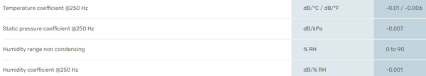
Figure 1—GRAS 46AE ½” free-field microphone environmental specifications taken from the GRAS website.
Environmental coefficients are typically divided into three aspects:
- Temperature.
- Humidity.
- Static pressure.
In an ideal world, measurement microphones have flat, stable frequency responses and sensitivities no matter the environmental conditions. In reality, though, due to how measurement microphones work, how they are manufactured, and the materials used in the capsules and preamplifier electronics, performance depends on environmental conditions.
IEC 61094 parts 1 and 4 describe the specifications for laboratory and working standard measurement microphones. The tolerances, including deviation limits due to changes in environmental conditions, are specified there.
Environmental coefficients describe the behavior of the microphone´s sensitivity under environmental conditions that differ from the reference conditions used during the microphone´s calibration in the lab. The reference environmental conditions are typically included in the microphone’s calibration certificate.
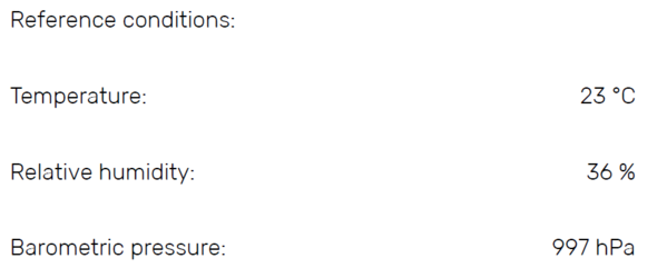
Figure 2—Example of GRAS 46AE reference environmental conditions extracted from a calibration chart.
Environmental coefficients are useful because it is possible to predict how the sensitivity of the microphone will change based on the real-world environmental conditions at the test site. It is also useful to understand if the measured sensitivity change when performing a field calibration is related to environmental factors or other things. However, they are mostly useful if there is a change in environmental conditions during the measurement. So, if the microphone is calibrated before starting the measurement and the environmental conditions change during the test, the accuracy of our measured data will decrease if the data is not corrected for the change.
It is also important to know that some calibration devices such as pistonphones will also need to be corrected for environmental conditions. So, it is always a good idea to check the pistonphone or calibrator manual to see if or how the performance of the reference signal is affected by the environmental conditions. Figure 3 shows an example of the pressure corrections needed pistonphone like GRAS 42AA or 42AP.
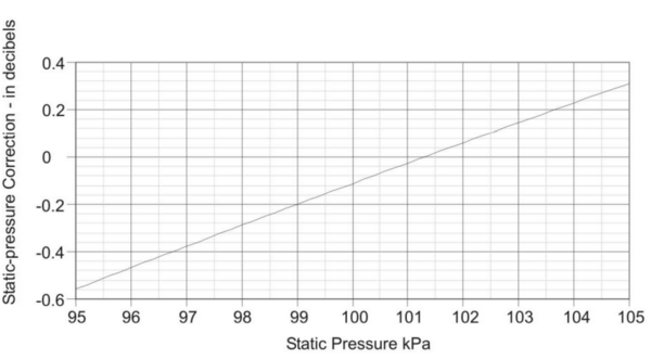
Figure 3—Static pressure corrections for a GRAS 42AA/AP Pistonphone.
Should changes always be assessed?
Of course, not all users have the same need regarding accuracy, so it is always important to assess when it is necessary to consider the environmental coefficients. Some applications also require tighter tolerances in respect to the accepted uncertainty of test results. For example, a calibration laboratory that is calibrating a sensor or calculating the uncertainty budget of a measurement signal chain will have different needs than an R&D engineer who is trying to perform a quick measurement to get fast results for a test. Also, other elements of a measurement signal chain or setup can add a greater uncertainty to the measurement than the sensitivity deviation in the sensor due to environmental conditions. For example, if the uncertainty of the sensitivity calibration of a sensor is +/-0.5 dB, then a possible sensitivity change of 0.01 dB due to temperature change may be considered negligible.
Environmental coefficients given in specifications provide typical values measured at a single frequency (e.g., 250Hz or 1kHz). In reality, each microphone will have a slightly different coefficient and the coefficient might not be the same for the entire frequency range. This is because the environmental condition changes can affect the sensitivity of the microphone in different ways depending on the frequency. Figure 4 shows an example of how the frequency response of a ¼″ pressure microphone is affected depending on the temperature. Higher frequencies (above about 6 kHz) are more affected by an increase or decrease in temperature compared to lower frequencies. Larger deviations are found around a microphone´s resonance frequency (around 40 kHz for the example.
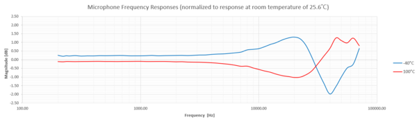
Figure 4—Microphone frequency response depending on temperature.
Figure 5 shows an example of the difference between the sensitivity variation at 250 Hz due to temperature change for two ¼″ pressure microphones of the same type.
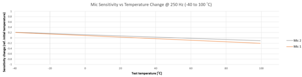
Figure 5—Microphone sensitivity variation due to temperature change for two ¼” pressure measurement microphones. IEC 61094-4 WS3P Temp Coef Tolerances: -0.03 to +0.03 (-10 to 50 °C); MIc. 1 Temp Coef. -0.0029 dB/°C (-40 to 100 °C); Mic. 2 Temp Coef. -0.00228 dB/°C (-40 to 100 °C)
It is important to mention that despite the small differences, shown in the example, both microphones’ temperature coefficients are way within the tolerances specified by IEC 61094-4 (Measurement Microphones: Specifications for Working Standard Microphones).
If a user is interested in knowing the exact environmental coefficients for a specific microphone, GRAS Lab offers the service of measuring its environmental coefficients. This can be useful for users looking for the ultimate accuracy and low uncertainty in their test results.
An example: Using the coefficients
Given a scenario with a GRAS 46AE ½” free-field measurement microphone in a setup where the temperature will fluctuate between 25 and 35˚C during a test, and give the calibration chart shown in Figure 6...
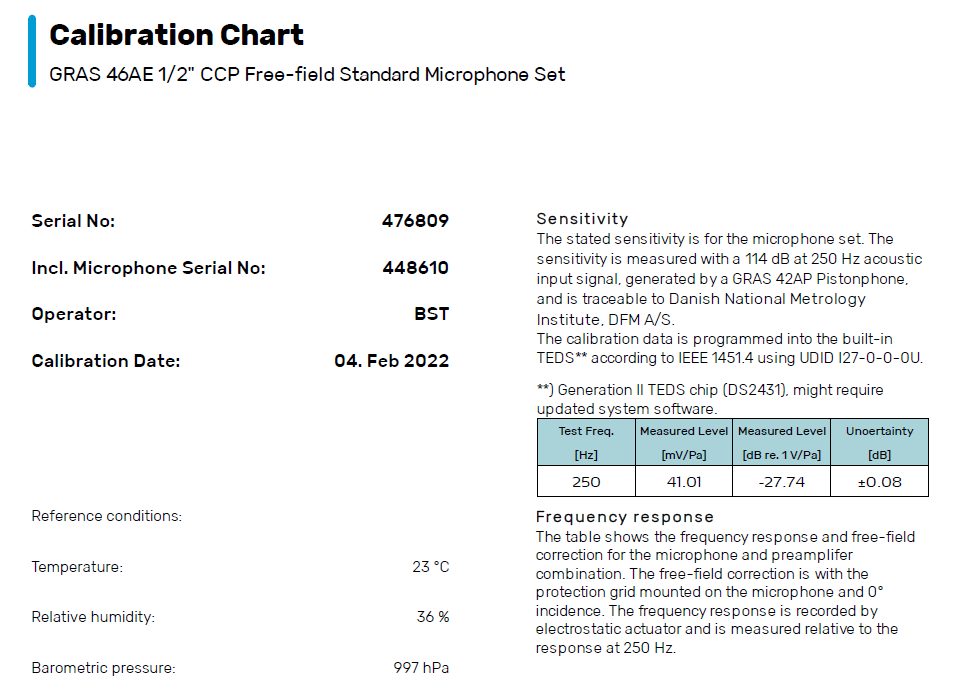
Figure 6—GRAS 46AE ½” free-field microphone calibration chart showing the close circuit sensitivity for the set (blue box) and environmental reference conditions (red box).
You can then apply a temperature coefficient correction as follows:
- Identify the type of microphone used. , both the microphone capsule and microphone set (mic + preamp combination) name will work. In this example, a GRAS 46AE microphone set is configured with a GRAS 40AE ½” free-field microphone capsule.
- On the GRAS website, search for the name of the microphone capsule or microphone set and check the environmental coefficients in the specifications section. The temperature coefficient for 46AE/40AE is -0.01 dB/˚C.
- Check the digital or paper version of the calibration chart for your specific microphone or microphone set´s sensitivity and environmental reference conditions (see Fig. 6). The environmental coefficients are typically expressed in dB, so work with the sensitivity in dB as well. (27.74 dB (re. 1V/Pa) for the 46AE in Figure 6).
- Calibrate the sensor using a sound calibrator or pistonphone before the start of a measurement. The sensitivity of a microphone may have changed slightly over the years or could differ from the calibration chart due to different environmental conditions (such as static pressure, temperature, or humidity). For this scenario, sensitivity is measured at -27.6 dB (re. 1V/Pa) @250Hz.
- Given the start (25 ˚C and the final temperature (35 ˚C) difference is 10˚C, the correction can be calculated as follows:
Temperature Correction [dB] = Temp. coefficient x (Final Temp – Start Temp)
Temperature Correction [dB] = -0.01 dB/˚C x (35 – 25 ˚C)
Temperature Correction [dB] = -0.1 dB
Which gives an expected sensitivity change (at 35 ˚C) of:
Sensitivity change [dB] = Original Sensitivity + Temperature correction
Sensitivity change [dB] = -27.6 dB + (-0.1) dB
Sensitivity change [dB] = -27.7 dB (re. 1V/Pa)
This means that the sensitivity of the microphone will decrease due to the increase in temperature, correlating with the example shown in Figure 4.
Conclusion
While different measurement scenarios have different needs regarding accuracy, and it is not always necessary to consider the environmental coefficients, they can have a considerable impact on measurements that have tight tolerances. Correct application of environmental coefficients enables the prediction of how the sensitivity changes due to real-world environmental fluctuations, especially those that occur during measurement. And the accurate application of sensitivity is one more stage in acquiring accurate data.
GRAS 46AE ½″ free-field microphone environmental specifications taken from the GRAS website.